A Friendly Introduction to Cross-Entropy Loss
By Rob DiPietro – Version 0.1 – May 2, 2016
Post or Jupyter Notebook?
This work is available both as a post and as a Jupyter notebook. If you see any mistakes or have any questions, please open a GitHub issue.
Introduction

When we develop a model for probabilistic classification, we aim to map the model's inputs to probabilistic predictions, and we often train our model by incrementally adjusting the model's parameters so that our predictions get closer and closer to ground-truth probabilities.
In this post, we'll focus on models that assume that classes are mutually exclusive. For example, if we're interested in determining whether an image is best described as a landscape or as a house or as something else, then our model might accept an image as input and produce three numbers as output, each representing the probability of a single class.
During training, we might put in an image of a landscape, and we hope that our model produces predictions that are close to the ground-truth class probabilities $y = (1.0, 0.0, 0.0)^T$. If our model predicts a different distribution, say $\hat{y} = (0.4, 0.1, 0.5)^T$, then we'd like to nudge the parameters so that $\hat{y}$ gets closer to $y$.
But what exactly do we mean by "gets closer to"? In particular, how should we measure the difference between $\hat{y}$ and $y$?
This post describes one possible measure, cross entropy, and describes why it's reasonable for the task of classification.
Entropy

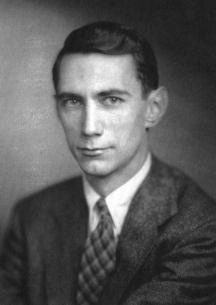
Claude Shannon
Let's say you're standing next to a highway in Boston during rush hour, watching cars inch by, and you'd like to communicate each car model you see to a friend. You're stuck with a binary channel through which you can send 0 or 1, and it's expensive: you're charged $0.10 per bit.
You need many bit sequences, one for each car model.
How would you allocate bit sequences to the car models? Would you use the same number of bits for the Toyota Camry sequence as you would for the Tesla Model S sequence?
No, you wouldn't. You'd allocate less bits to the Camry, because you know that you'll end up sending the Camry sequence much more often than the Tesla Model S sequence. What you're doing is exploiting your knowledge about the distribution over car models to reduce the number of bits that you need to send on average.
It turns out that if you have access to the underlying distribution $y$, then to use the smallest number of bits on average, you should assign $\log \frac{1}{y_i}$ bits to the $i$-th symbol. (As a reminder, $y_i$ is the probability of the $i$-th symbol.)
For example, if we assume that seeing a Toyota is 128x as likely as seeing a Tesla, then we'd give the Toyota symbol 7 less bits than the Tesla symbol:
$$ b_\mbox{toyota} = \log \frac{1}{128 p_\mbox{tesla}} = \log \frac{1}{p_\mbox{tesla}} + \log \frac{1}{128} = b_\mbox{tesla} - 7 $$By fully exploiting the known distribution $y$ in this way, we achieve an optimal number of bits per transmission. The optimal number of bits is known as entropy. Mathematically, it's just the expected number of bits under this optimal encoding:
$$ H(y) = \sum_i y_i \log \frac{1}{y_i} = -\sum_i y_i \log y_i $$Cross Entropy

If we think of a distribution as the tool we use to encode symbols, then entropy measures the number of bits we'll need if we use the correct tool $y$. This is optimal, in that we can't encode the symbols using fewer bits on average.
In contrast, cross entropy is the number of bits we'll need if we encode symbols from $y$ using the wrong tool $\hat{y}$. This consists of encoding the $i$-th symbol using $\log \frac{1}{\hat{y}_i}$ bits instead of $\log \frac{1}{y_i}$ bits. We of course still take the expected value to the true distribution $y$, since it's the distribution that truly generates the symbols:
$$ H(y, \hat{y}) = \sum_i y_i \log \frac{1}{\hat{y}_i} = -\sum_i y_i \log \hat{y}_i $$Cross entropy is always larger than entropy; encoding symbols according to the wrong distribution $\hat{y}$ will always make us use more bits. The only exception is the trivial case where $y$ and $\hat{y}$ are equal, and in this case entropy and cross entropy are equal.
KL Divergence

The KL divergence from $\hat{y}$ to $y$ is simply the difference between cross entropy and entropy:
$$ \mbox{KL}(y~||~\hat{y}) = \sum_i y_i \log \frac{1}{\hat{y}_i} - \sum_i y_i \log \frac{1}{y_i} = \sum_i y_i \log \frac{y_i}{\hat{y}_i} $$It measures the number of extra bits we'll need on average if we encode symbols from $y$ according to $\hat{y}$; you can think of it as a bit tax for encoding symbols from $y$ with an inappropriate distribution $\hat{y}$. It's never negative, and it's 0 only when $y$ and $\hat{y}$ are the same.
Note that minimizing cross entropy is the same as minimizing the KL divergence from $\hat{y}$ to $y$. (They're equivalent up to an additive constant, the entropy of $y$, which doesn't depend on $\hat{y}$.)
Predictive Power

After our discussion above, maybe we're happy with using cross entropy to measure the difference between two distributions $y$ and $\hat{y}$, and with using the total cross entropy over all training examples as our loss. In particular, if we let $n$ index training examples, the overall loss would be
$$ H(\{y^{(n)}\}, \{\hat{y}^{(n)}\}) = \sum_n H(y^{(n)}, \hat{y}^{(n)}) $$But let's look at another approach.
What if we want our objective function to be a direct measure of our model's predictive power, at least with respect to our training data?
One common approach is to tune our parameters so that the likelihood of our data under the model is maximized. Since for classification we often use a discriminative model, our "data" often just consists of the labels we're trying to predict. A model that often predicts the ground-truth labels given the inputs might be useful; a model that often fails to predict the ground-truth labels isn't useful.
Because we usually assume that our samples are independent and identically distributed, the likelihood over all of our examples decomposes into a product over the likelihoods of individual examples:
$$ L(\{y^{(n)}\}, \{\hat{y}^{(n)}\}) = \prod_n L(y^{(n)}, \hat{y}^{(n)}) $$And what's the likelihood of the $n$-th example? It's just the particular entry of $\hat{y}^{(n)}$ that corresponds to the ground-truth label specified by $y^{(n)}$!
Going back to the original example, if the first training image is of a landscape, then $y^{(1)} = (1.0, 0.0, 0.0)^T$, which tells us that the likelihood $L(y^{(1)}, \hat{y}^{(1)})$ is just the first entry of $\hat{y}^{(1)} = (0.4, 0.1, 0.5)^T$, which is $\hat{y}^{(1)}_1 = 0.4$.
To keep going with this example, let's assume we have a total of four training images, with labels {landscape, something else, landscape, house}, giving us ground-truth distributions $y^{(1)} = (1.0, 0.0, 0.0)^T$, $y^{(2)} = (0.0, 0.0, 1.0)^T$, $y^{(3)} = (1.0, 0.0, 0.0)^T$, and $y^{(4)} = (0.0, 1.0, 0.0)^T$. Our model would predict four other distributions $\hat{y}^{(1)}$, $\hat{y}^{(2)}$, $\hat{y}^{(3)}$, and $\hat{y}^{(4)}$, and the overall likelihood would just be
$$ L(\{y^{(1)}, y^{(2)}, y^{(3)}, y^{(4)}\}, \{\hat{y}^{(1)}, \hat{y}^{(2)}, \hat{y}^{(3)}, \hat{y}^{(4)}\}) = \hat{y}^{(1)}_1 \, \hat{y}^{(2)}_3 \, \hat{y}^{(3)}_1 \, \hat{y}^{(4)}_2 $$Maybe the last section made us happy with minimizing cross entropy during training, but are we still happy?
Why shouldn't we instead maximize the likelihood $L(\{y^{(n)}\}, \{\hat{y}^{(n)}\})$ of our data?
Unified Loss

Let's play a bit with the likelihood expression above.
First, since the logarithm is monotonic, we know that maximizing the likelihood is equivalent to maximizing the log likelihood, which is in turn equivalent to minimizing the negative log likelihood
$$ -\log L(\{y^{(n)}\}, \{\hat{y}^{(n)}\}) = -\sum_n \log L(y^{(n)}, \hat{y}^{(n)}) $$But from our discussion above, we also know that the log likelihood of $y^{(n)}$ is just the log of a particular entry of $\hat{y}^{(n)}$. In fact, it's the entry $i$ which satisfies $y^{(n)}_i = 1.0$. We can therefore rewrite the log likelihood for the $n$-th training example in the following funny way:
$$ \log L(y^{(n)}, \hat{y}^{(n)}) = \sum_i y^{(n)}_i \log \hat{y}^{(n)}_i $$which gives us an overall negative log likelihood of
$$ - \log L(\{y^{(n)}\}, \{\hat{y}^{(n)}\}) = -\sum_n \sum_i y^{(n)}_i \log \hat{y}^{(n)}_i $$Starting to look familiar? This is precisely cross entropy, summed over all training examples:
$$ -\log L(\{y^{(n)}\}, \{\hat{y}^{(n)}\}) = \sum_n \big[-\sum_i y_i \log \hat{y}^{(n)}_i\big] = \sum_n H(y^{(n)}, \hat{y}^{(n)})$$Conclusions

When we develop a probabilistic model over mutually exclusive classes, we need a way to measure the difference between predicted probabilities $\hat{y}$ and ground-truth probabilities $y$, and during training we try to tune parameters so that this difference is minimized.
In this post we saw that cross entropy is a reasonable choice.
From one perspective, minimizing cross entropy lets us find a $\hat{y}$ that requires as few extra bits as possible when we try to encode symbols from $y$ using $\hat{y}$.
From another perspective, minimizing cross entropy is equivalent to minimizing the negative log likelihood of our data, which is a direct measure of the predictive power of our model.
Acknowledgements
The entropy discussion is based on Andrew Moore's slides. The photograph of Claude Shannon is from Wikipedia. All other photographs were obtained from pixabay.
I'd also like to thank my advisor, Gregory D. Hager, for being supportive of this work.
About Me

GitHub Twitter
I'm Rob DiPietro, a PhD student in the Department of Computer Science at Johns Hopkins, where I'm advised by Gregory D. Hager. For more information and/or tutorials, please visit https://rdipietro.github.com.
Subscribe
I rarely post new projects / tutorials, but sign up if you'd like to hear about them when I do: